Step by step linear regression example
In this article we will try out linear regression on Boston data set. As we go forward in the course, we shall include more complexities.
As a first step, let us check for outliers and high leverage points.
dt %>%
  pivot_longer(cols = c(1:14)) %>%
  ggplot(aes(x=value))+
  geom_boxplot()+
  facet_wrap(~name)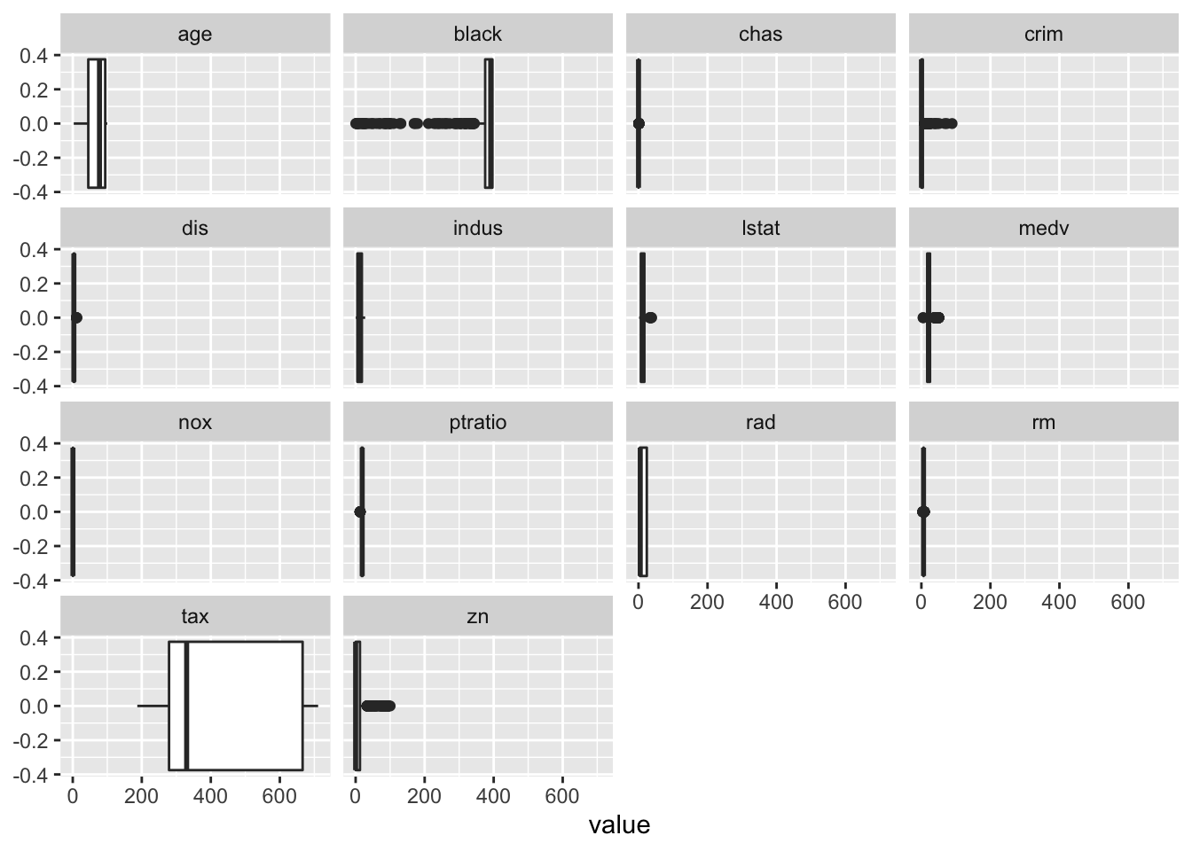
It looks like some of the variables have substantial number of outliers. Well, in this case, we will not consider them as outliers. Outliers are usually just a few points away from the data. In our case, it is not so. Moreover, removing these will remove a lot of data. As we go forward, we shall try to find out ways to tackle this. For now, we will keep the variable.
Next we will look for collinearity.
psych::corPlot(dt[1:13])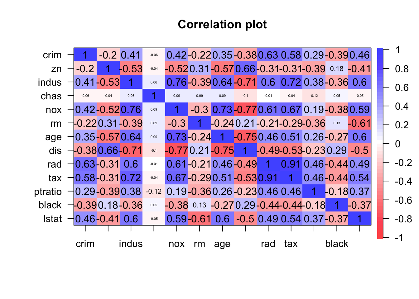
Some heavy correlations are noticed.
We can remove nox,age, dis and tax.
dt.new<-dt %>%
  dplyr::select(-c(nox,dis,tax,age))

psych::corPlot(dt.new)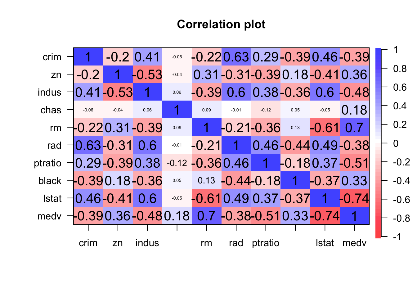
How about multicollinearity? We will calculate the variation inflation factor for that
fit1<-lm(medv~., data=dt.new)
car::vif(fit1)
## crim zn indus chas rm rad ptratio black
## 1.764273 1.522811 2.296931 1.051265 1.759611 2.501243 1.515956 1.336424
## lstat
## 2.461788As a thumb rule, vif <=4 is acceptable. All the values are within acceptable range.
Now let us work on improving the model.
summary(fit1)##
## Call:
## lm(formula = medv ~ ., data = dt.new)
##
## Residuals:
## Min 1Q Median 3Q Max
## -18.3213 -2.9803 -0.8391 1.6229 29.0234
##
## Coefficients:
## Estimate Std. Error t value Pr(>|t|)
## (Intercept) 13.821352 4.353376 3.175 0.001592 **
## crim -0.074061 0.034909 -2.122 0.034369 *
## zn -0.004990 0.011961 -0.417 0.676710
## indus -0.024030 0.049941 -0.481 0.630612
## chas 3.141969 0.912558 3.443 0.000624 ***
## rm 4.535619 0.426793 10.627 < 2e-16 ***
## rad 0.096209 0.041060 2.343 0.019518 *
## ptratio -0.951894 0.128565 -7.404 5.71e-13 ***
## black 0.010732 0.002863 3.749 0.000198 ***
## lstat -0.521405 0.049670 -10.497 < 2e-16 ***
## ---
## Signif. codes: 0 '***' 0.001 '**' 0.01 '*' 0.05 '.' 0.1 ' ' 1
##
## Residual standard error: 5.08 on 496 degrees of freedom
## Multiple R-squared: 0.7003, Adjusted R-squared: 0.6949
## F-statistic: 128.8 on 9 and 496 DF, p-value: < 2.2e-16Seems like zn and indus do not add value to the model.
fit2<-update(fit1,~. -zn-indus)
summary(fit2)
##
## Call:
## lm(formula = medv ~ crim + chas + rm + rad + ptratio + black +
## lstat, data = dt.new)
##
## Residuals:
## Min 1Q Median 3Q Max
## -18.3932 -3.0253 -0.8268 1.5912 28.9649
##
## Coefficients:
## Estimate Std. Error t value Pr(>|t|)
## (Intercept) 13.320540 4.239152 3.142 0.001776 **
## crim -0.074051 0.034786 -2.129 0.033764 *
## chas 3.119025 0.900617 3.463 0.000580 ***
## rm 4.547522 0.423947 10.727 < 2e-16 ***
## rad 0.090037 0.038412 2.344 0.019471 *
## ptratio -0.942444 0.124456 -7.572 1.79e-13 ***
## black 0.010822 0.002849 3.798 0.000164 ***
## lstat -0.524916 0.046935 -11.184 < 2e-16 ***
## ---
## Signif. codes: 0 '***' 0.001 '**' 0.01 '*' 0.05 '.' 0.1 ' ' 1
##
## Residual standard error: 5.071 on 498 degrees of freedom
## Multiple R-squared: 0.7002, Adjusted R-squared: 0.6959
## F-statistic: 166.1 on 7 and 498 DF, p-value: < 2.2e-16Now, if we want to improve this model further, we may want to include some non-linear transformation. That the data is non-linear can be verified from residual plot
ggplot(fit2, aes(x = .fitted, y = .resid)) +
  geom_point()+
    labs(
    title ="Residual Plot",
    subtitle = "Funnel not observed, but pattern observed",
    y="Residuals",
    x="fitted Values"
  ) +
  theme_ft_rc()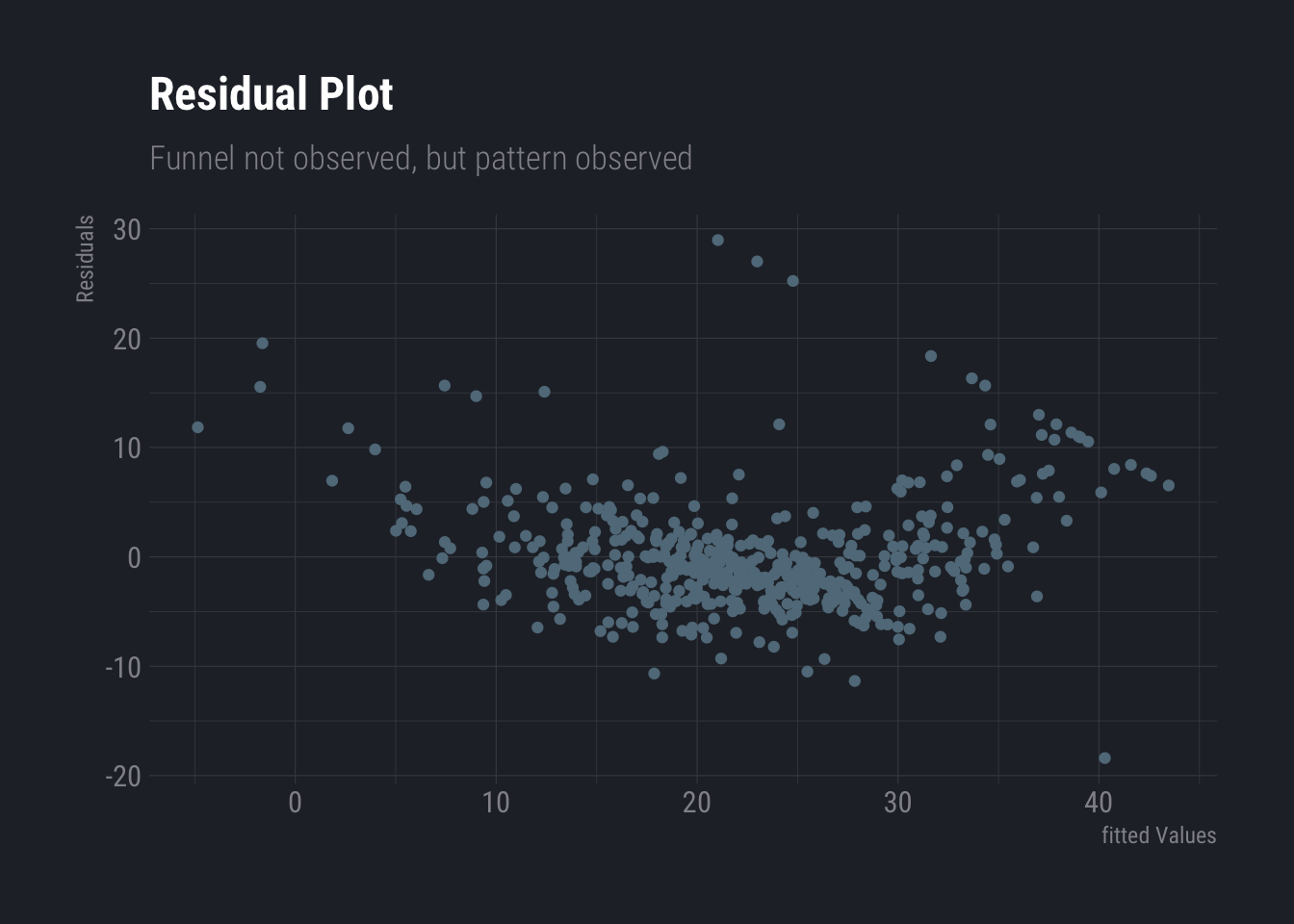
Before try transformations, we may want to explore which variable is perhaps best suitable for transformation.
dt.new %>%
  dplyr::select(-c(zn,indus)) %>%
  pivot_longer(cols=c(crim:lstat)) %>%
  ggplot(aes(x=medv, y=value))+
  geom_point()+
  facet_wrap(~name, scales="free")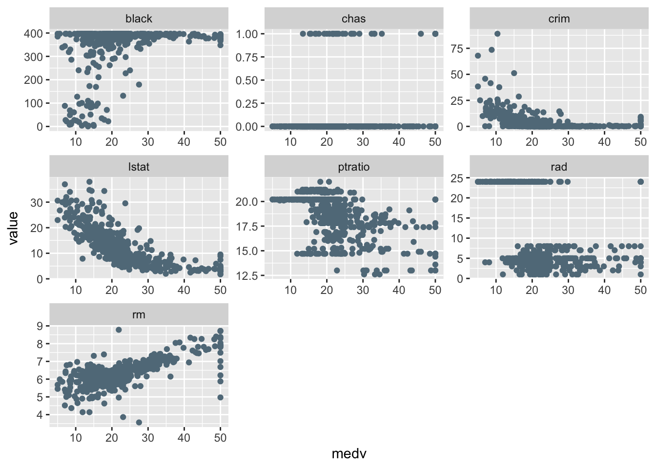
It seems there is some scope in lstat and I will give a try in crim, ptratio and black as well.
fit3<-lm(medv~chas+rm+rad+crim+ptratio+black+poly(lstat,2), data=dt.new)
summary(fit3)
##
## Call:
## lm(formula = medv ~ chas + rm + rad + crim + ptratio + black +
## poly(lstat, 2), data = dt.new)
##
## Residuals:
## Min 1Q Median 3Q Max
## -19.6624 -2.5796 -0.5902 2.0314 27.0008
##
## Coefficients:
## Estimate Std. Error t value Pr(>|t|)
## (Intercept) 8.045020 3.617897 2.224 0.026619 *
## chas 3.215190 0.819548 3.923 9.97e-05 ***
## rm 3.832808 0.392046 9.776 < 2e-16 ***
## rad 0.120163 0.035076 3.426 0.000664 ***
## crim -0.123788 0.032024 -3.865 0.000126 ***
## ptratio -0.748036 0.114832 -6.514 1.79e-10 ***
## black 0.009204 0.002598 3.543 0.000432 ***
## poly(lstat, 2)1 -94.386333 6.925106 -13.630 < 2e-16 ***
## poly(lstat, 2)2 49.729480 4.865249 10.221 < 2e-16 ***
## ---
## Signif. codes: 0 '***' 0.001 '**' 0.01 '*' 0.05 '.' 0.1 ' ' 1
##
## Residual standard error: 4.615 on 497 degrees of freedom
## Multiple R-squared: 0.7522, Adjusted R-squared: 0.7482
## F-statistic: 188.6 on 8 and 497 DF, p-value: < 2.2e-16After few attempts, I selected the above model
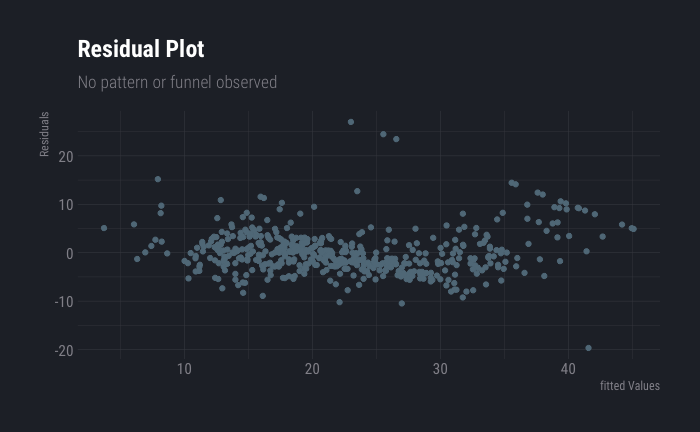
Next we check the residual plot again. The pattern is less visible (compared to last residual plot). Heteroscedasticity is also not observed.
ggplot(fit3, aes(x = .fitted, y = .resid)) +
geom_point()+
labs(
title ="Residual Plot",
subtitle = "No pattern or funnel observed",
y="Residuals",
x="fitted Values"
) +
theme_ft_rc()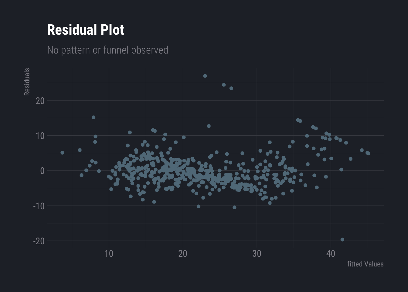 Before we end this section, we also check for correlations in error terms. Looks like there could be a slight correlation which can be ignored.
ggplot(data.frame(resi=fit3$residuals, ind=as.integer(names(fit3$residuals))), aes(x=ind,y=resi))+
  geom_line(aes(x=ind,y=resi))+
  geom_point() +
      labs(
    title ="Residual Plot",
    subtitle = "Possibility of slight correlation in error terms are observed",
    y="Residuals",
    x="Index"
  ) +
  theme_ft_rc()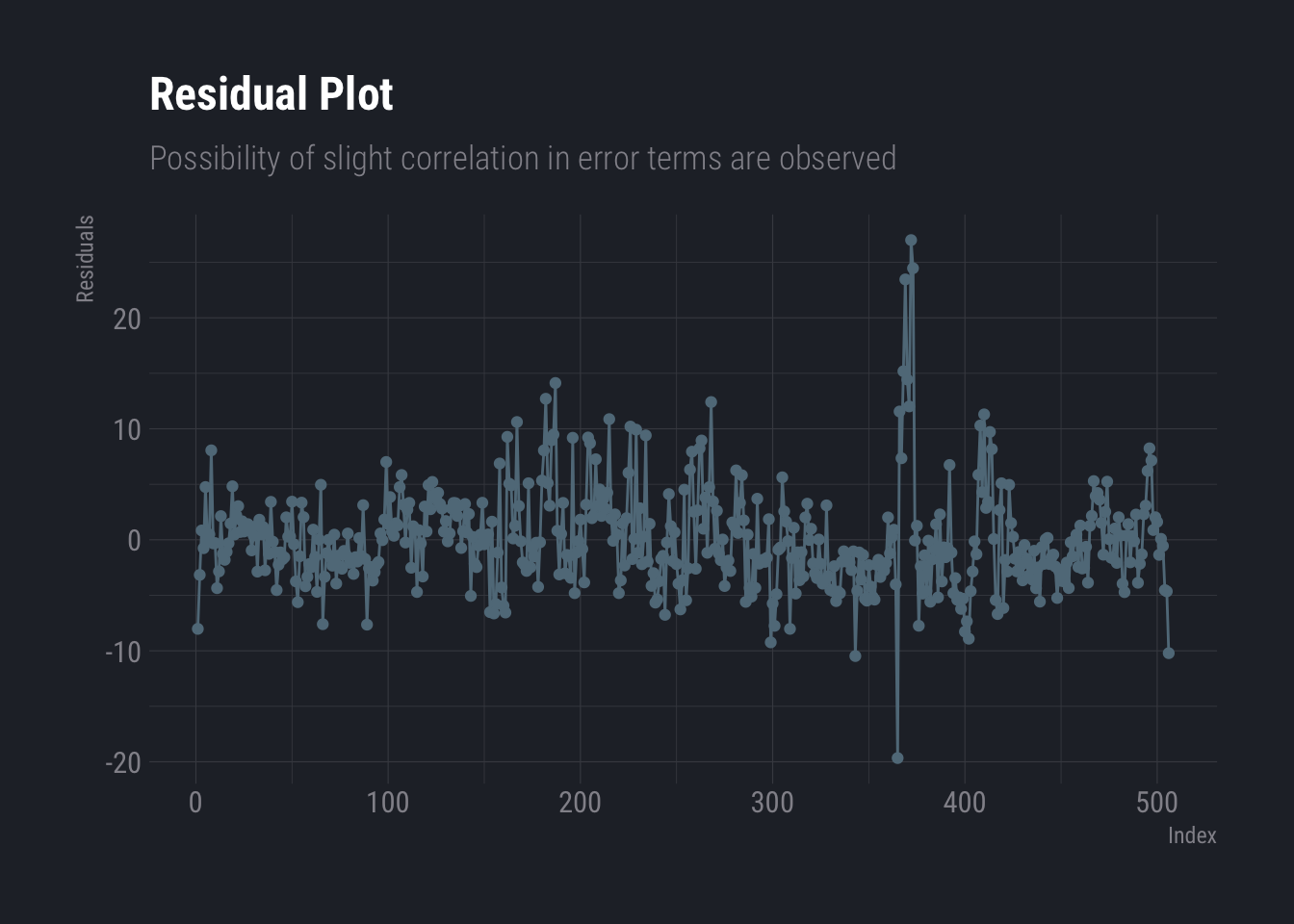
So, our final model is as follows
summary(fit3)##
## Call:
## lm(formula = medv ~ chas + rm + rad + crim + ptratio + black +
## poly(lstat, 2), data = dt.new)
##
## Residuals:
## Min 1Q Median 3Q Max
## -19.6624 -2.5796 -0.5902 2.0314 27.0008
##
## Coefficients:
## Estimate Std. Error t value Pr(>|t|)
## (Intercept) 8.045020 3.617897 2.224 0.026619 *
## chas 3.215190 0.819548 3.923 9.97e-05 ***
## rm 3.832808 0.392046 9.776 < 2e-16 ***
## rad 0.120163 0.035076 3.426 0.000664 ***
## crim -0.123788 0.032024 -3.865 0.000126 ***
## ptratio -0.748036 0.114832 -6.514 1.79e-10 ***
## black 0.009204 0.002598 3.543 0.000432 ***
## poly(lstat, 2)1 -94.386333 6.925106 -13.630 < 2e-16 ***
## poly(lstat, 2)2 49.729480 4.865249 10.221 < 2e-16 ***
## ---
## Signif. codes: 0 '***' 0.001 '**' 0.01 '*' 0.05 '.' 0.1 ' ' 1
##
## Residual standard error: 4.615 on 497 degrees of freedom
## Multiple R-squared: 0.7522, Adjusted R-squared: 0.7482
## F-statistic: 188.6 on 8 and 497 DF, p-value: < 2.2e-16Later in the course, we shall try to improve it further.