Confidence Interval and Hypothesis Testing
Confidence Interval
In a way the idea of inferential statistics (and machine learning) revolve around estimation of population characteristics from sample. Often the estimation is incorrectly calculated as a single point. For example, one may take a random sample of customers in a shop and calculate the average amount they spent. Let us assume that amount is x. One may use this number (x) as the population mean. This however, may be highly unreliable. While estimation of population parameter from sample parameter, there is always probability involved, as we had noticed in the article on sampling distribution. Hence, it is always better to provide the estimates as interval with a confidence interval.
Confidence interval for single population mean when population standard deviation is known
Suppose a random survey of 300 Netflix users reveal that they spend 78 minutes on Netflix. And the population standard deviation is known and is 21 minutes. To estimate the true mean, we first decide on the level of confidence or probability. Let us say that we want to be 95 % confident.
This 78 minutes corresponds to a certain position or z-stat in its distribution. And the 95 % also provides another z-stat.
95 % confidence interval defines two boundaries. In this specific case, the 95 % is calculated as the middle 95 %. In other cases it may be 95 % from the left or right. These boundaries have specific and defined z-scores. z-scores for the 2.5 % and 97.5 % can be obtained from z-table. In modern statistical software, there are functions which can calculate these for you.
# Z score for 2.5 %
qnorm(0.025)
## [1] -1.959964# Z score for 97.5 %
qnorm(0.975)## [1] 1.959964These standard z-scores are calculated assuming mean of 0 and standard deviation of 1. However, in our population (and sample) mean is not 0 and standard deviation is not 1. Therefore, we need to transform this z-score into a measure of scale that relates to the variable of interest.
This is usually done by
\[ z = \frac{\bar x - \mu}{\frac{\sigma}{\sqrt(n)}} \]
where \(\bar x\) is sample mean, \(\mu\) is population mean, n is number of samples, \(\sigma\) is the population standard deviation. The denominator is called sampling error.
So, the population mean range equals
lower_range=78+qnorm(0.025)*(21/sqrt(300))
upper_range=78-qnorm(0.025)*(21/sqrt(300))
data.frame(lower_range,upper_range)
## lower_range upper_range
## 1 75.62367 80.37633In practice, seldom does anyone come across problems where population standard deviation is know. Hence, there is no in built function in R to calculate the confidence interval with known population standard deviation. However, one can create their own function as shown below
ci.norm<- function(data, variance = var(data), conf.level = 0.95) {
  z.score = qnorm((1 - conf.level)/2, lower.tail = FALSE)
  sam.mean = mean(data)
  sd.error = sqrt(variance/length(data))
  c(sam.mean - z.score * sd.error, sam.mean + z.score * sd.error)
}
library(ggplot2)
# library(hrbrthemes)
# import_roboto_condensed()
ggplot() +
geom_density(aes(x=rnorm(1000))) +
geom_vline(aes(xintercept=qnorm(0.025))) +
geom_vline(aes(xintercept=qnorm(0.975))) +
geom_segment(aes(x=qnorm(0.025), xend=-qnorm(0.025), y=0.2, yend=0.2), arrow = arrow(ends = "both", length = unit(0.5,"cm"))) +
geom_text(aes(x=0, y=0.21, label="95%")) +
geom_text(aes(x=2.3, y=0.06, label="97.5% \n 80.37")) +
geom_text(aes(x=-2.3, y=0.06, label="2.5% \n 75.62")) +
labs(title = "Confidence interval calculation",
x="Variable values",
y="Density")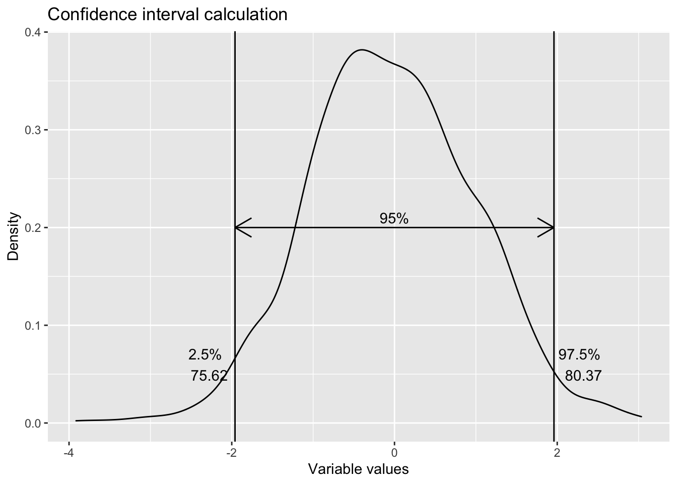
Trade off between confidence and precision
| Confidence Interval | z - scores | Formula |
|---|---|---|
| 90 % | ~1.64, ~-1.64 | \(\bar x \pm 1.64 \frac{\sigma}{\sqrt n}\) |
| 95 % | ~ 1.96, ~- 1.96 | \(\bar x \pm 1.96 \frac{\sigma}{\sqrt n}\) |
| 99 % | ~2.58, ~ -2.58 | \(\bar x \pm 2.58 \frac{\sigma}{\sqrt n}\) |
The table above shows the different z scores (ranges) at different confidence intervals and then the corresponding formula. It may be noticed that as confidence interval increases, the interval or the range of possible parameter value also increases. That means, when we try to increase confidence, we decrease precision and vice-versa.
It may also me noticed that if n i.e. the sample size is increased, the range decreases i.e. the precision increases.
How is it actually applied?
Suppose that you are aware of the population mean. You can calculate a confidence interval that will cover the possible sample means. Similarly, when you take samples, each of them will have confidence intervals. Let us assume that 5 samples were taken for an analysis. The plot below shows them.
ggplot() +
  geom_density(aes(x=rnorm(1000,78,21))) +
  geom_vline(aes(xintercept=qnorm(0.025, 78,21))) +
  geom_vline(aes(xintercept=qnorm(0.975, 78,21))) +
  geom_segment(aes(x=qnorm(0.025, 78,21), xend=qnorm(0.975, 78,21), y=0.005, yend=0.005), arrow = arrow(ends = "both", length = unit(0.5,"cm"))) +
  geom_vline(aes(xintercept=78))+
  geom_text(aes(x=120, y=0.0006, label="97.5%")) +
  geom_text(aes(x=72, y=0.0053, label="Population Mean (95% C I)"))+
  geom_text(aes(x=40, y=0.0006, label="2.5%")) +
  geom_segment(aes(x=c(50,50, 120, 100, 40), xend=c(70, 100, 130, 130, 90), y=c(0.012,0.015,0.0075,0.0025,0.02),
                   yend=c(0.012,0.015,0.0075,0.0025,0.02)), arrow = arrow(ends = "both", length = unit(0.5,"cm")))+
  geom_text(aes(x=c(50,50, 120, 100, 40), y= c(0.013, 0.016, 0.0076, 0.0026, 0.021), label=c("Sample 1", "Sample 2", "Sample 3", "Sample 4", "Sample 5")))+
  labs(title = "Confidence interval calculation",
       x="Variable values",
       y="Density")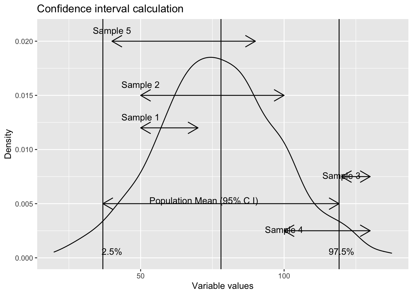
The samples whose confidence interval range fall, even partially, mean that their (sample) means are not a representative of the population mean. In our example, since the confidence interval considered in 95 %, we can expect that 5 % of the time, the sample means will fall beyond the limit (despite being a randomly selected sample).
Confidence interval, when population standard deviation is unknown
When population standard deviation is not known, we use t-score. The basic concept remains same but the calculations differ a bit (In standard error calculation, since we do not know the population mean, sample mean in used).
In R, there is a straightforward function t.test() that can easily calculate this for you.
Confidence interval for population proportion
Confidence interval calculation also follows the same logic, albeit, the formula is different. The basic difference is in calculation of standard error. Instead of standard deviation, p(1-p) is used in the numerator, where p is the sample proportion.
These concepts form the base to apply hypothesis testing.
Hypothesis Testing
Hypothesis testing is used to validate (or reject) claim of a population parameter, based on observed sample parameter. The population parameters are the central tendencies - mean, proportions, difference of means and difference of proportions.
The first step in hypothesis testing is formulating the null hypothesis (and hence, the alternative hypothesis as well). This is followed by determining the region of acceptance of the null hypothesis. Then sample test statistic (for example z-stat or z-score) is calculated and observed if it falls within the acceptable range calculated in the previous step. Usually null hypothesis represents the status quo. It always contains an equality sign (equal to, greater or equal to and smaller or equal to). Hypothesis tests are of three types.
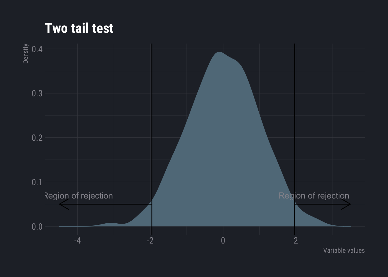
- Two sided Whenever the test is for equality, two sided tests are used. H0 : Population parameter = Some value (This is the null hypothesis) H1 : Population parameter \(\not=\) That value (This is the alternative hypothesis)
ggplot() +
  geom_density(aes(x=rnorm(1000))) +
  geom_vline(aes(xintercept=qnorm(0.025))) +
  geom_vline(aes(xintercept=qnorm(0.975))) +
  geom_segment(aes(x=c(qnorm(0.025),qnorm(0.975)), xend=c(-4.5,3.5), y=c(0.05,0.05), yend=c(0.05,0.05)), arrow = arrow(ends = "last", length = unit(0.5,"cm")))+
  geom_text(aes(x=c(-4, 2.5), y=c(0.07,0.07), label=c("Region of rejection","Region of rejection")) )+
  labs(title = "Two tail test",
       x="Variable values",
       y="Density")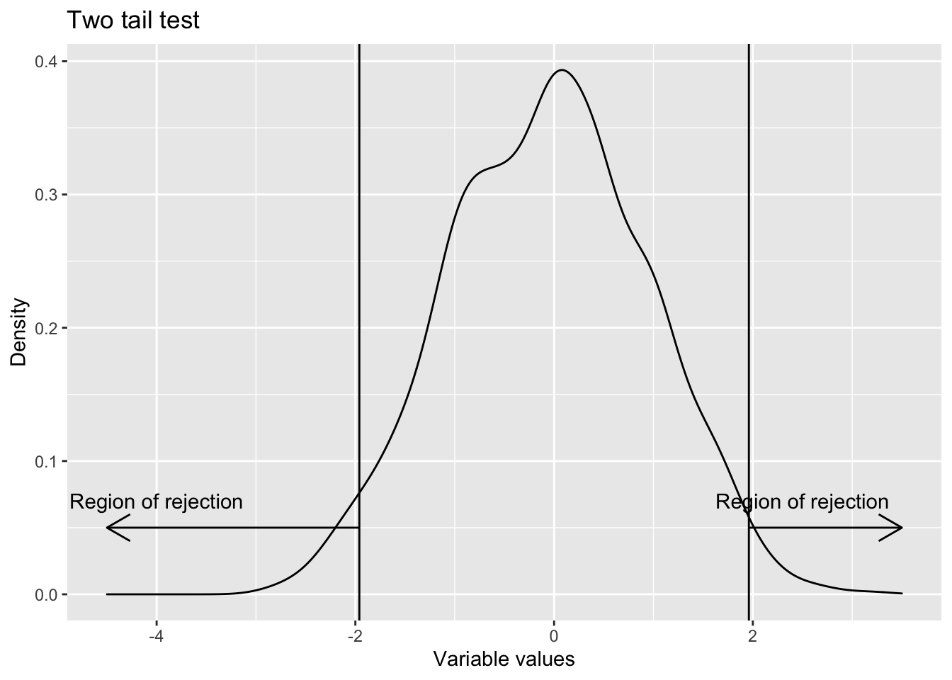
- One sided upper tail Whenever the test is for more than some value (i.e the claim is that population parameter is more than some value), upper tail test is used. H0 : Population parameter \(\leq\) Some value (This is the null hypothesis) H1 : Population parameter > That value (This is the alternative hypothesis)
ggplot() +
  geom_density(aes(x=rnorm(1000))) +
  #geom_vline(aes(xintercept=qnorm(0.025))) +
  geom_vline(aes(xintercept=qnorm(0.975))) +
  geom_segment(aes(x=c(qnorm(0.975)), xend=c(3.5), y=c(0.05), yend=c(0.05)), arrow = arrow(ends = "last", length = unit(0.5,"cm")))+
  geom_text(aes(x=c(2.5), y=c(0.07), label=c("Region of rejection")) )+
  labs(title = "Upper tail test",
       x="Variable values",
       y="Density")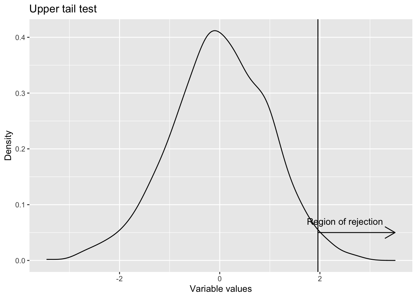
- One sided lower tail Whenever the test is for less than or equal to (i.e. the claim is that population parameter is less than some value), lower tail test is used. H0 : Population parameter \(\geq\) Some value (This is the null hypothesis) H1 : Population parameter < That value (This is the alternative hypothesis)
ggplot() +
  geom_density(aes(x=rnorm(1000))) +
  geom_vline(aes(xintercept=qnorm(0.025))) +
  geom_segment(aes(x=c(qnorm(0.025)), xend=c(-4.5), y=c(0.05), yend=c(0.05)), arrow = arrow(ends = "last", length = unit(0.5,"cm")))+
  geom_text(aes(x=c(-4), y=c(0.07), label=c("Region of rejection")) )+
  labs(title = "Lower tail test",
       x="Variable values",
       y="Density")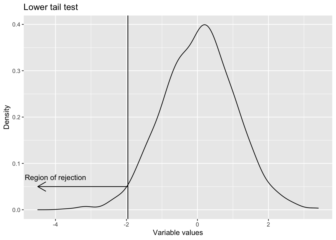
As you might have realized that these tests carry some risk of wrong prediction. Type I error is the the probability of rejecting the null hypothesis when it is actually true. And Type II is one where null hypothesis is accepted when it is actually incorrect. Reducing one, increases the other.
Type I errors are also called the level of significance. It is, in fact, the area under curve of the rejection region. When we set this area, we obtain the limit that separates the acceptance region from the rejection region. This limit (or limits) is (or are) called critical limits and the statistic at those points are called critical statistic. For example, z-crit or t-crit.
Once we have the z-crit or t-crit , we find the z-stat from the sample. If z-stat falls within the acceptance region defined by z-crit or t-crit, we accept the null hypothesis. Else, we reject it.
Hypothesis testing examples
Single population mean with known standard deviation
This is almost never happen in real live. Nonetheless, it shall be explained here, using an example. Let us assume that the a store a store manager thinks that average purchase value in her store is $1000. It is known that the population standard deviation is 200. The manager wants to not test if her assumption is correct. So she takes a sample of 300 customers and the mean sample mean is $750.
So, out hypotheses are
Ho: Population mean = $1000 H1: Population mean \(\not =\) $1000
Let us say we want the level of significance (\(\alpha\)) to be 5%. So, z-crit is \(\pm 1.96\). Let us calculate the test statistic. For the null hypothesis to hold true, the test statistic should be between -1.96 and 1.96.
pop.mean.assumed=1000
sample.mean=750
pop.sd= 200
sample.size= 300

standard.error=pop.sd/sqrt(sample.size)

z.stat=(pop.mean.assumed-sample.mean)/standard.error

z.stat
## [1] 21.65064This z.stat is miles away from the z-crit calculated earlier. Hence, we can reject the null hypothesis, in favour of the alternative.
Single population mean with unknown standard deviation
Since this kind of problem is often encountered in real life, R has an inbuilt function to calculate this. Let us assume that we have sample weights from some students in a class. And we want to understand if the population mean is
- equal to 45
- less than 45 and
- greater than 45
All three examples are shown below
sample.values<-c(42,56,29,35,47,37,39,29,45,35,51,53)

# If null hypothesis = population mean in 45
t.test(x = sample.values,mu = 45,alternative = c("two.sided"),conf.level =0.95)
##
## One Sample t-test
##
## data: sample.values
## t = -1.3411, df = 11, p-value = 0.2069
## alternative hypothesis: true mean is not equal to 45
## 95 percent confidence interval:
## 35.75606 47.24394
## sample estimates:
## mean of x
## 41.5The result shows that the population mean is estimated to be between 35.7 and 47.24. So, the null hypothesis is not rejected. This is also visible in the p-value. We would have rejected it, had it been less than 0.05.
Two other hypotheses are tested below.
# If null hypothesis = population mean <= 45
t.test(x = sample.values,mu = 45,alternative = c("less"),conf.level =0.95)
##
## One Sample t-test
##
## data: sample.values
## t = -1.3411, df = 11, p-value = 0.1035
## alternative hypothesis: true mean is less than 45
## 95 percent confidence interval:
## -Inf 46.18675
## sample estimates:
## mean of x
## 41.5# If null hypothesis = population mean >= 45
t.test(x = sample.values,mu = 45,alternative = c("greater"),conf.level =0.95)##
## One Sample t-test
##
## data: sample.values
## t = -1.3411, df = 11, p-value = 0.8965
## alternative hypothesis: true mean is greater than 45
## 95 percent confidence interval:
## 36.81325 Inf
## sample estimates:
## mean of x
## 41.5Similarly, we can use the function prop.test() to test for proportions.
Multiple population
Suppose you want to compare means of two populations. And you want to do that using samples from each of the populations. It can be easily calculated as shown below.
x =c(70,82,78,74,94,82)

y =c(64,72,60,76,72,80,84,68)

t.test(x, y,alternative =c("two.sided"),var.equal =TRUE)
##
## Two Sample t-test
##
## data: x and y
## t = 1.8234, df = 12, p-value = 0.09324
## alternative hypothesis: true difference in means is not equal to 0
## 95 percent confidence interval:
## -1.559502 17.559502
## sample estimates:
## mean of x mean of y
## 80 72Since, the range of the possible difference the population mean is estimated to be between -1.5 and 17.5 and 0 lies between these two numbers, we cannot reject the null hypothesis (that the difference in mean equals 0 or the means are equal).
Notice that I have assumed equal variance in both the populations. If that is not the case, it can be changed. There are some tests that can be used to check if the variance can be assumed to be equal or not (F-test). But, we will skip it for now.
Sometimes, you want to test the difference on the same population before and after some event. For example, if you want to check if a medicine works or not or if a training has been successful or not. So, whenever we have a before and after situation, we use matched pair t test. We can use the same function by changing the parameter paired to TRUE.
before <-rnorm(10,100,3)
after <-rnorm(10,110,3)

t.test(before, after, paired = TRUE, alternative = "two.sided")
##
## Paired t-test
##
## data: before and after
## t = -9.1043, df = 9, p-value = 7.769e-06
## alternative hypothesis: true difference in means is not equal to 0
## 95 percent confidence interval:
## -14.182081 -8.537041
## sample estimates:
## mean of the differences
## -11.35956Similar approach can be taken in testing proportions as well using prop.test() function.
Chi squared test
Chi squared test is used to test for independence. For example is the choice of color associated with buyers gender? It can be also used to test for equality of proportions. For example is the percentage of females equal across fortune 500 companies? Finally, it can also be used to check for goodness of fit. For example, are weights of students normally distributed?
Say you three colours of balls in a huge bag. You want to understand if occurrence of each colored ball is equal.
ball.color.count<-c(81, 50, 27)
chisq.test(ball.color.count)
##
## Chi-squared test for given probabilities
##
## data: ball.color.count
## X-squared = 27.886, df = 2, p-value = 8.803e-07Since p values is less than 0.05, we reject the null hypothesis that the proportions are equal.
In this example we tested for equality. We can even define the exact probabilities.
chisq.test(ball.color.count, p=c(4/7,2/7,1/7))##
## Chi-squared test for given probabilities
##
## data: ball.color.count
## X-squared = 2.3465, df = 2, p-value = 0.3094In this case, we cannot reject the null hypothesis. Please notice the new probabilities provided, which are not equal.
To test goodness of fit, one needs to provide the probabilities and values. Suppose we have a set of random values a (see below). And we want to check its goodness of fit with a normal distribution with mean 3 and sd 2 (see b below).
a<-rnorm(n=10,mean=7,sd=2)

b<-pnorm(seq(0.1,1,by=0.1), mean=3,sd=2)

chisq.test(x=a,p=b, rescale.p=T)
## Warning in chisq.test(x = a, p = b, rescale.p = T): Chi-squared approximation
## may be incorrect##
## Chi-squared test for given probabilities
##
## data: a
## X-squared = 9.6089, df = 9, p-value = 0.3831As expected, we cannot reject the null hypothesis (That they fit), i.e. the sample and the distribution does not fit.
In another example, assume that you want to check if gender and smoking habit are independent of each other.
dt <- matrix(c(120, 90, 40, 110, 95, 45), ncol=3, byrow=TRUE)

rownames(dt)<-c("male","female")
colnames(dt)<-c("non_smoker","occ_smoker","chain_smoker")
dt<-as.table(dt)
And we have a sample of data as shown above. To test independence, we can use the same method.
chisq.test(dt)##
## Pearson's Chi-squared test
##
## data: dt
## X-squared = 0.86404, df = 2, p-value = 0.6492Here, we can say that row and column variables are not significantly associated because p value is not less than 0.5.
I have mentioned p-value quite often. P-value is the area under the curve from the test statistic to the end of the curve.
I strongly recommend you to go through the following video to understand further.
And this for a walk through in R.